Towards Exascale Computing

1. Introduction

Over the past ten years, my research journey has revolved around one central question: how can we design finite element algorithms that are accurate, scalable, and fast enough to solve real-world scientific and engineering problems?

In this talk, I want to share how my work in finite element analysis gradually moved toward high-performance computing, cloud computing, and now exascale computing.

I will not go too deep into the mathematics or scientific details. Instead, I want to focus on the challenges, the lessons, and the opportunities that exist in this field.

My intent is simple: to inspire students, researchers, and engineers to enter this area and contribute to the advancement of scientific simulations.

Scientific computing is still far from solving many real-world problems at the fidelity we would like. That means there is a lot of room for new ideas, new algorithms, and new researchers.

2. Research Journey So Far

My actual research journey started during my high school days. I come from a small town in Himachal Pradesh, India. During my schooling at Him Academy Public School in Hamirpur, I was introduced to the scientific method and computer programming.

Later, I moved to NIT Raipur to pursue my bachelor’s degree in civil engineering. This is where I was first introduced to simulations, specifically civil engineering simulations. Towards the end of my undergraduate studies, I developed a complete 3D finite element analysis package.

After that, I was selected to work as a scientist at the Department of Atomic Energy in Mumbai. At the same time, I was also selected for my master’s at IIT Roorkee. The Department of Atomic Energy allowed me to continue my master’s in structural engineering at IIT Roorkee and sponsored my studies.

That is how I started working on nuclear structural problems.

After completing my master’s, I joined the Department of Atomic Energy and worked on the analysis and design of nuclear power plant structures. Later, I returned to IIT Roorkee for my PhD, where I focused on understanding and designing finite element algorithms that could give accurate solutions in the minimum possible time.

After completing my PhD, I moved to the United States for a NASA-funded project on algorithms for cloud computing systems. Today, I am working as an Assistant Professor at Vanderbilt University, continuing this journey toward large-scale and exascale computing.

3. Inspiration to Start PhD

The inspiration for my PhD came from my time at BARC.

At BARC, I was working in the civil engineering department. We had to interact with multiple vendors and several internal departments, including mechanical, electrical, and civil teams (see Fig.1).

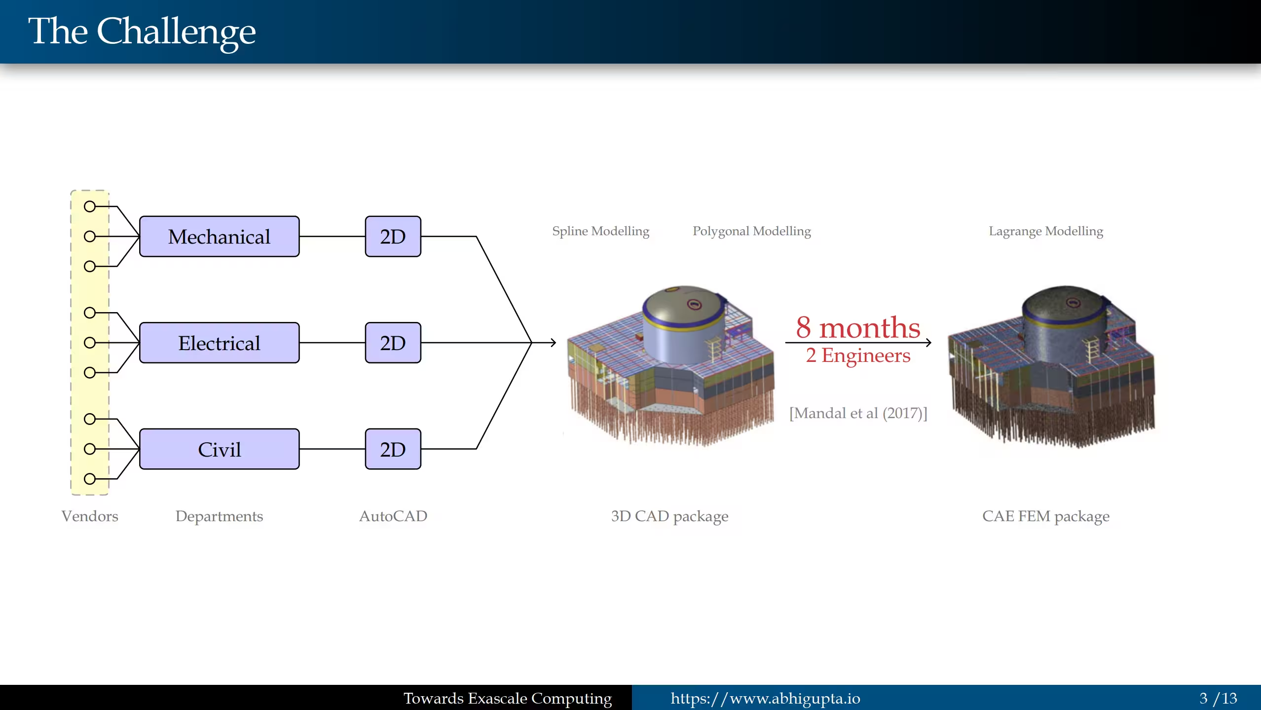Figure 1: The challenge that inspired me to do a PhD

These teams would provide their specifications, which then had to be converted into 2D engineering drawings. These 2D drawings were then converted into a 3D CAD model, and finally, the CAD model was converted into a finite element model.

This entire process could take months, sometimes even years. The bigger problem was that if there was any change in the pipeline, we had to redo a large part of the process.

Once we finally had the 3D finite element model, it still took around a month to solve all the static and dynamic analyses for a huge nuclear reactor model.

That was the problem I wanted to solve.

I kept asking myself: why does it take a month to get a solution? Why can’t we get it in a day, or even in an hour?

That question pushed me back toward research. I wanted to understand finite element algorithms at a deeper level and design methods that could produce accurate solutions faster.

4. Research Limits During COVID

At the start of my PhD, I had a very simple setup: an iMac with 8 GB RAM and an Intel i5 processor with six cores. This was not a high-performance computing system, but I started building finite element algorithms from scratch on it.

I was able to solve small two-dimensional academic problems such as dendrite solidification, mechanical topology optimization, thermo-mechanical topology optimization, and dynamic fracture simulations (see Fig. 2).

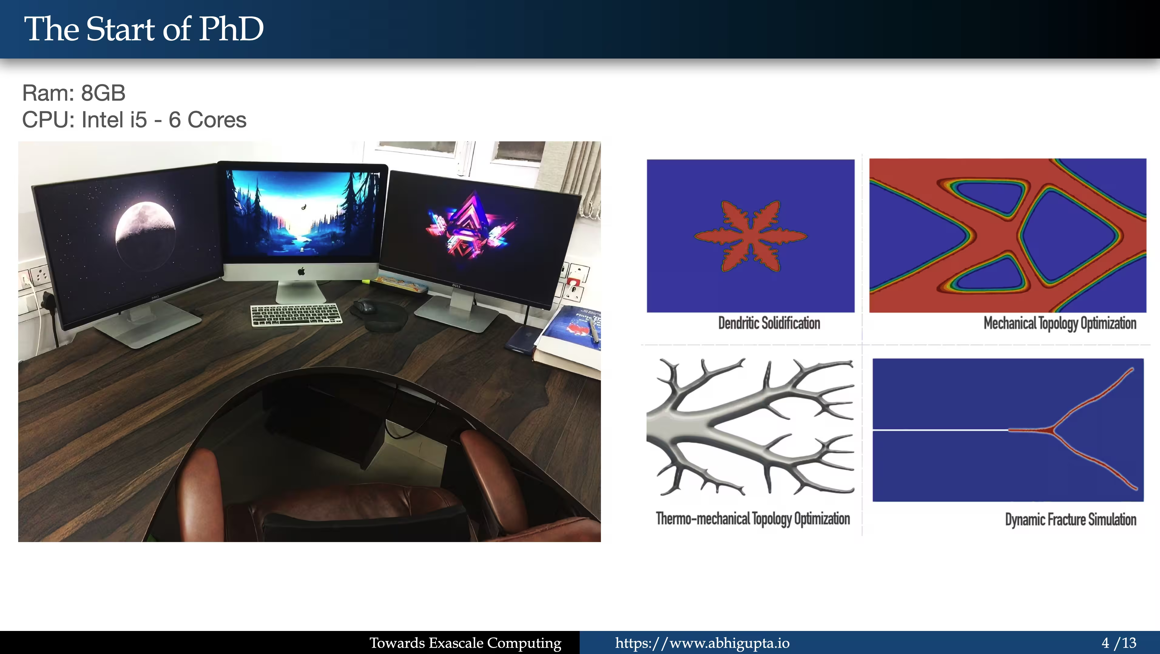Figure 2: Solving 2D academic problems on an i5 processing computer

These problems had tens of thousands, or at most hundreds of thousands, of degrees of freedom. They could still be handled on 8 GB of RAM.

But actual industry-grade problems are not that small. They require millions or billions of degrees of freedom and much larger computing systems.

During COVID, all institutions were shut down. We lost access to the large servers and computing resources at our institution. I was left with my laptop, and I had no way to run the large-scale simulations I had hoped to work on.

That limitation forced me to think more deeply about the computational cost of finite element analysis.

To get more accurate solutions, we usually increase the size of the system. We add more degrees of freedom, and the solution gets closer to reality. But we cannot increase the system size indefinitely because we are limited by memory and computational resources.

In finite element analysis, the cost of algorithms grows roughly as $n^α$. Here, $n$ is the size of the system and $\alpha$ depends on several mathematical and algorithmic choices (see Fig. 3).

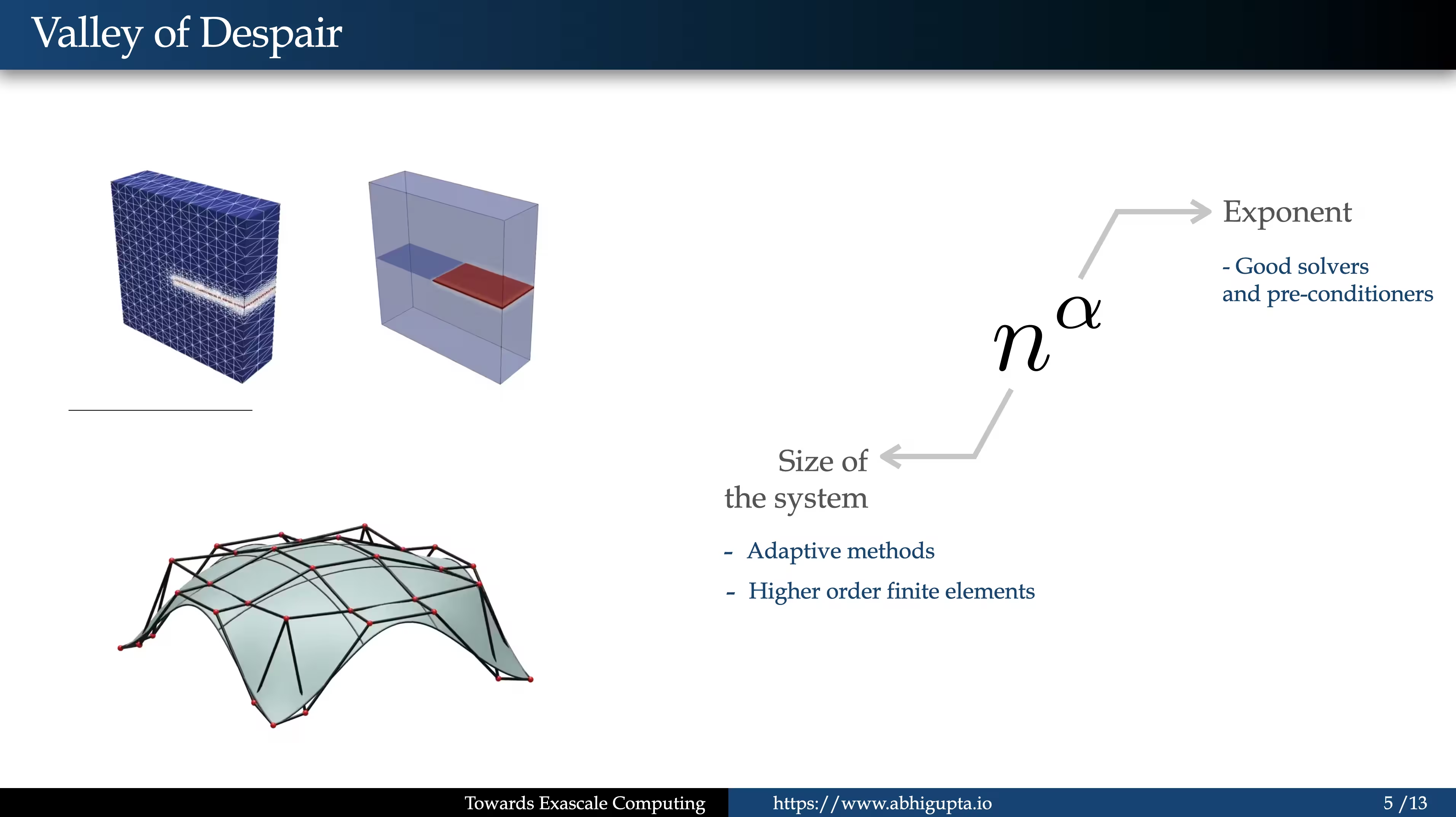Figure 3: Cost of algorithm depending on $n^{\alpha}$

One important realization was that we should not always refine the entire domain. For fracture problems, the quantity of interest is often local: the fracture path. So instead of refining the whole model, we can refine only the region around the crack.

Using adaptive methods, we could achieve the desired accuracy while keeping the number of degrees of freedom under control. In one case, instead of using tens of millions of degrees of freedom, we could solve the problem with under $100,000$ degrees of freedom. That directly reduced the runtime by a huge factor.

Another approach was to use higher-order finite elements, such as isogeometric analysis. In one shape optimization problem, instead of using tens of thousands of degrees of freedom, I could get the solution with only $36$ degrees of freedom.

The lesson was clear: we should not simply brute-force problems with bigger and bigger systems. We need to understand the physics, the quantity of interest, and the numerical method. That is how we design better finite element algorithms.

5. Introduction to FEniCS Project

When the COVID shutdown was lifted, I was able to return to the larger systems at our institution. I had access to an HP Z4 workstation with 800 GB RAM and 96 cores. It was a powerful machine, and I could push it to its limits.

But I soon realized that coding everything from scratch and parallelizing everything manually in C++ or Python was too much work. There are excellent libraries and frameworks that can accelerate the development process.

One such library is the FEniCS Project.

FEniCS allows us to use available computing resources without worrying about every detail of parallelization. We can design the finite element algorithm inside the framework, and the framework can take advantage of the computing cores available on the system.

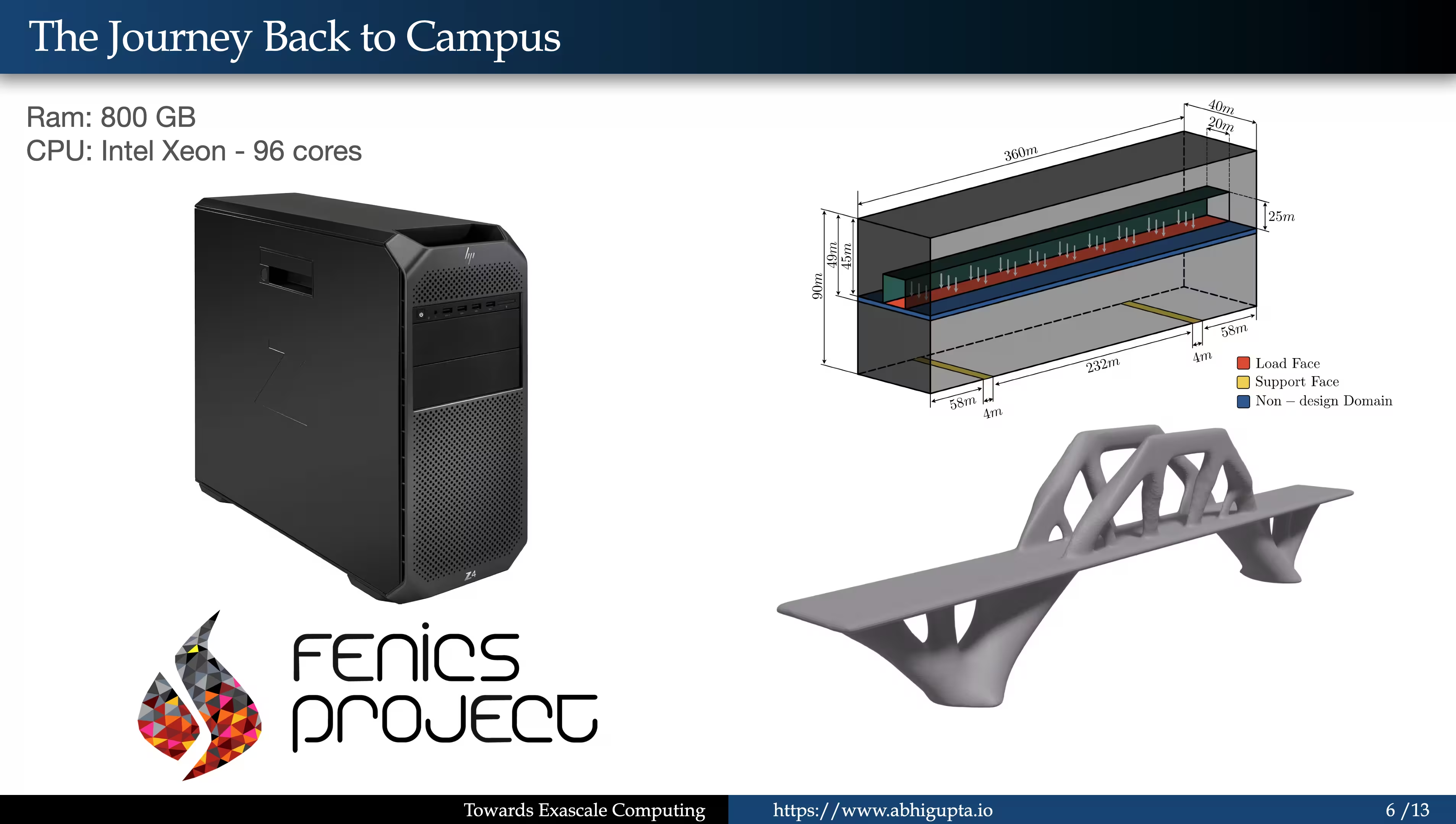Figure 4: Industry-scale topology optimization using FEniCS

However, not all problems need parallel computing. There is a size threshold. In my experience, you get real benefit from parallelization when you have at least around 50,000 degrees of freedom per core. If the problem is smaller than that, parallel computing may not be necessary.

With the workstation and FEniCS, I was able to solve industry-grade problems and push the system to more than 500 million degrees of freedom (see Fig. 4).

These were the kinds of simulations I had previously done with commercial packages during my time at BARC, but now I could recreate them using my own algorithms, with control over each component of the finite element pipeline.

6. Importance of Cloud Computing

After completing my PhD, I moved to the United States and started working on a NASA-funded project.

The problem involved glacier fracture simulation. On the left side of the Fig. 5, I showed an actual satellite image from NASA’s repository of the Larsen C Ice Shelf. On the right side, is finite element mesh generated directly on satellite images using a tool called Icepack, developed by my collaborators from Washington State University.

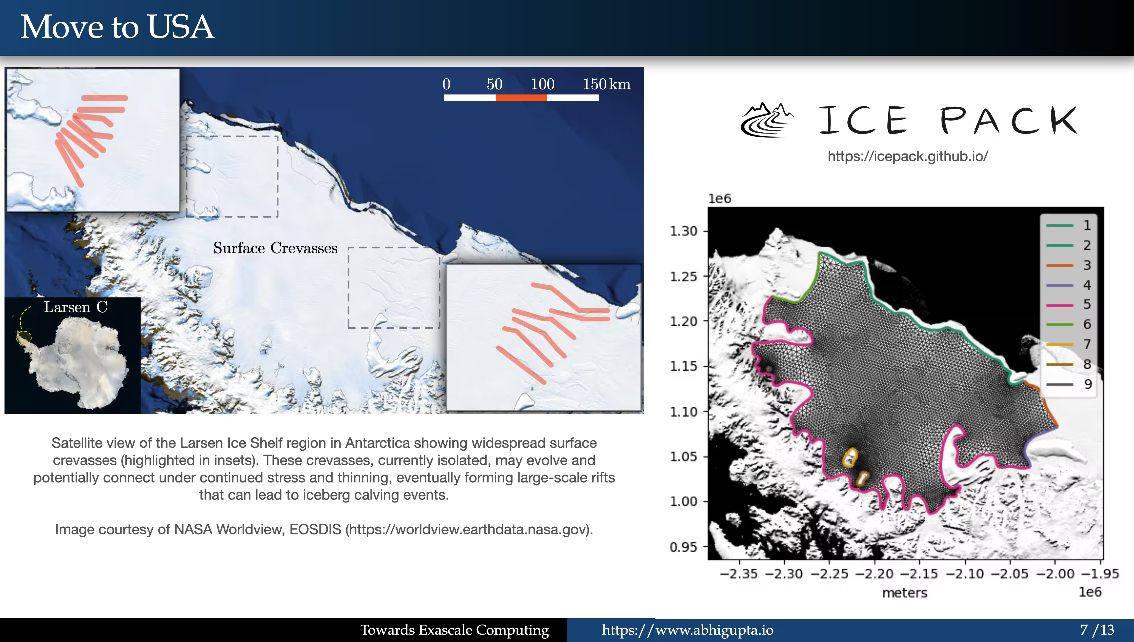Figure 5: Large scale problem of Larsen Ice Shelf region in Antarctica

This problem is truly large scale.

The ice sheet is hundreds of kilometers long, but the fracture we want to model may be only meters wide, or even centimeters wide. That creates a huge multiscale challenge.

A workstation with up to a terabyte of RAM can handle medium to large-scale problems. But to model fine-scale cracks in glaciers at meter or half-meter resolution, we would need trillions of degrees of freedom.

That is beyond what a normal workstation can handle.

This is where cloud computing becomes important. To solve billions or trillions of degrees of freedom, we either need institutional servers or we need to move to cloud computing.

7. Cloud Computing for Finite Simulations

I was fortunate to receive a grant from Google Cloud to work on this problem. We started building our algorithms and scaling them on Google Cloud instead of limiting ourselves to local workstations.

This is where frameworks like FEniCS or MFEM become very useful. Unlike many commercial packages, these frameworks give us fine-grained control over every component of the algorithm. That control allows us to tune the algorithm for the cloud computing resources we are using.

The way we approached it was by building a cluster of nodes. Think of it like having 100 machines in a computer lab and joining them together to solve a single problem. On Google Cloud, we can create such clusters and deploy our algorithms across them.

But this introduces new challenges.

Now we are not just splitting a problem across multiple CPU cores on one workstation. We are splitting it across multiple CPU cores and multiple machines. That means we need to understand CPUs, GPUs, RAM, networking, data storage, software libraries, and distributed computing.

At this scale, everything becomes complicated.

For example, if a workstation has 800 GB RAM and we store one iteration of the solution, the output itself can be huge. If the simulation has 1,000 time steps, the storage requirement can multiply by 1,000. Suddenly, we may need thousands of terabytes of storage.

In our glacier problem, we solved a sample block of ice of size 1.5 km by 0.75 km on Google Cloud. If we had fully refined the problem, it would have required around a billion degrees of freedom. Using adaptive methods, we solved it with around 13 million degrees of freedom and reduced the cost by roughly a factor of 100 (Fig. 6).

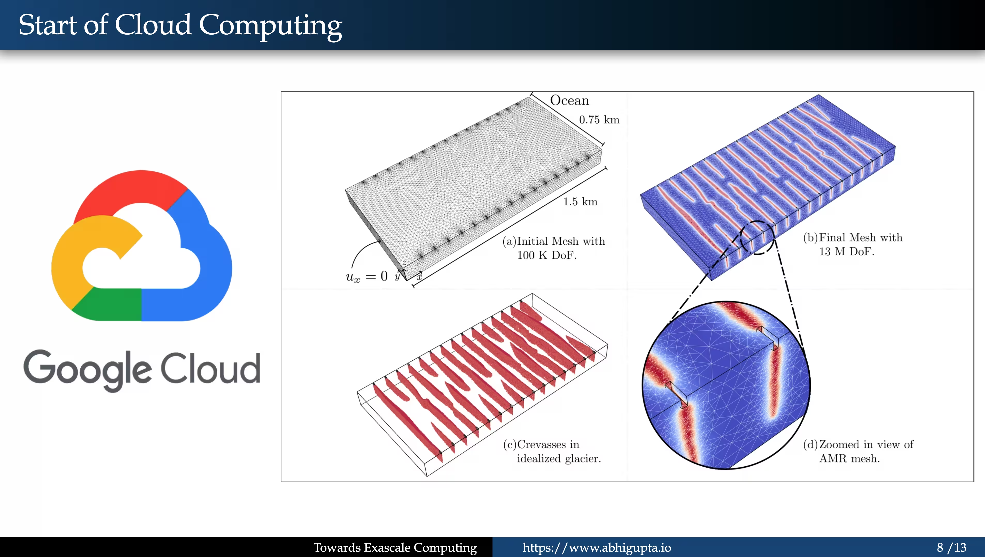Figure 6: Google cloud computing for solving Larcen Ice Shelf problem

This matters because cloud cost scales quickly. If a brute-force simulation costs a million dollars, better algorithms may bring that cost down to around $10,000.

That is the dream: better algorithms making large-scale scientific simulation economically feasible.

8. The Next Steps: Towards Exaflop

My journey started with a laptop that had 6 to 12 cores and around 16 GB RAM. Today, laptops can have up to 128 GB RAM and 12 to 24 cores. They may reach around 0.1 teraflops.

A workstation can have hundreds of cores and a few terabytes of RAM. It may reach around 20 teraflops.

But an exascale system like the Frontier supercomputer in Tennessee is on an entirely different scale. Frontier has around 8 million compute units and more than 9 million GB of combined memory. It can reach around two exaflops.

To explain this simply, imagine FLOPS as speed.

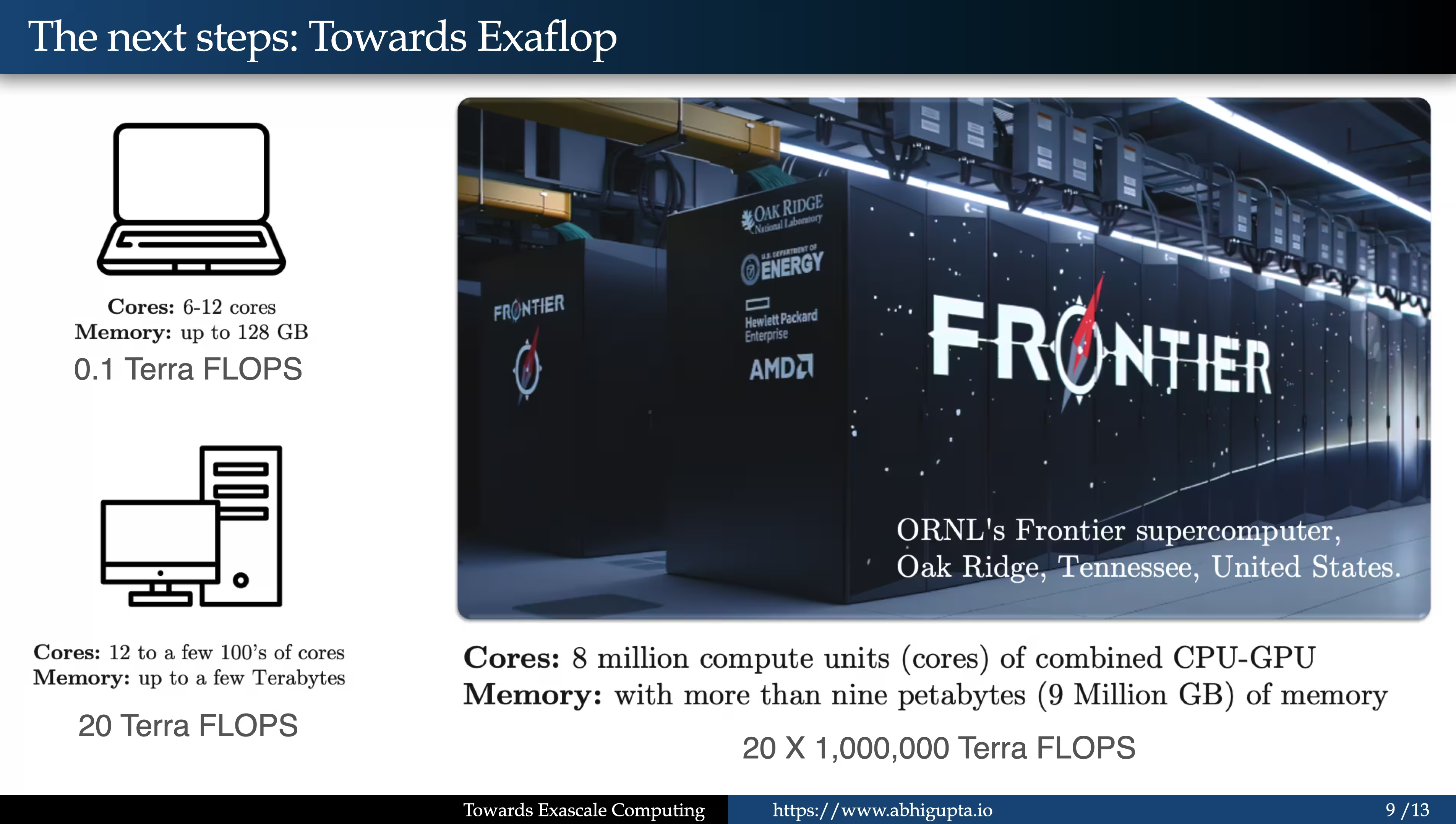Figure 7: Comparison of Flops with laptop, workstations, and super computers.

A laptop may be moving at 0.1 miles per hour. A workstation may move at 20 miles per hour. But an exascale system like Frontier may move at 20 million miles per hour (see Fig. 7).

Of course, these are theoretical peak speeds. To actually benefit from them, we need better algorithms and better software systems.

But the possibility is extraordinary. I have seen researchers solve problems with five trillion degrees of freedom and achieve speeds of around two exaflops. Problems that could take millions of years on smaller systems may become solvable in days or weeks.

These are the kinds of problems we want to solve with truly large-scale computing.

9. Next Challenges in Large-Scale Computing

Even with exascale systems, there are many challenges.

The first major challenge is meshing at scale. On a workstation, meshing a billion-degree-of-freedom problem may take one or two hours. But when we move to trillions of elements, generating high-quality meshes becomes extremely difficult.

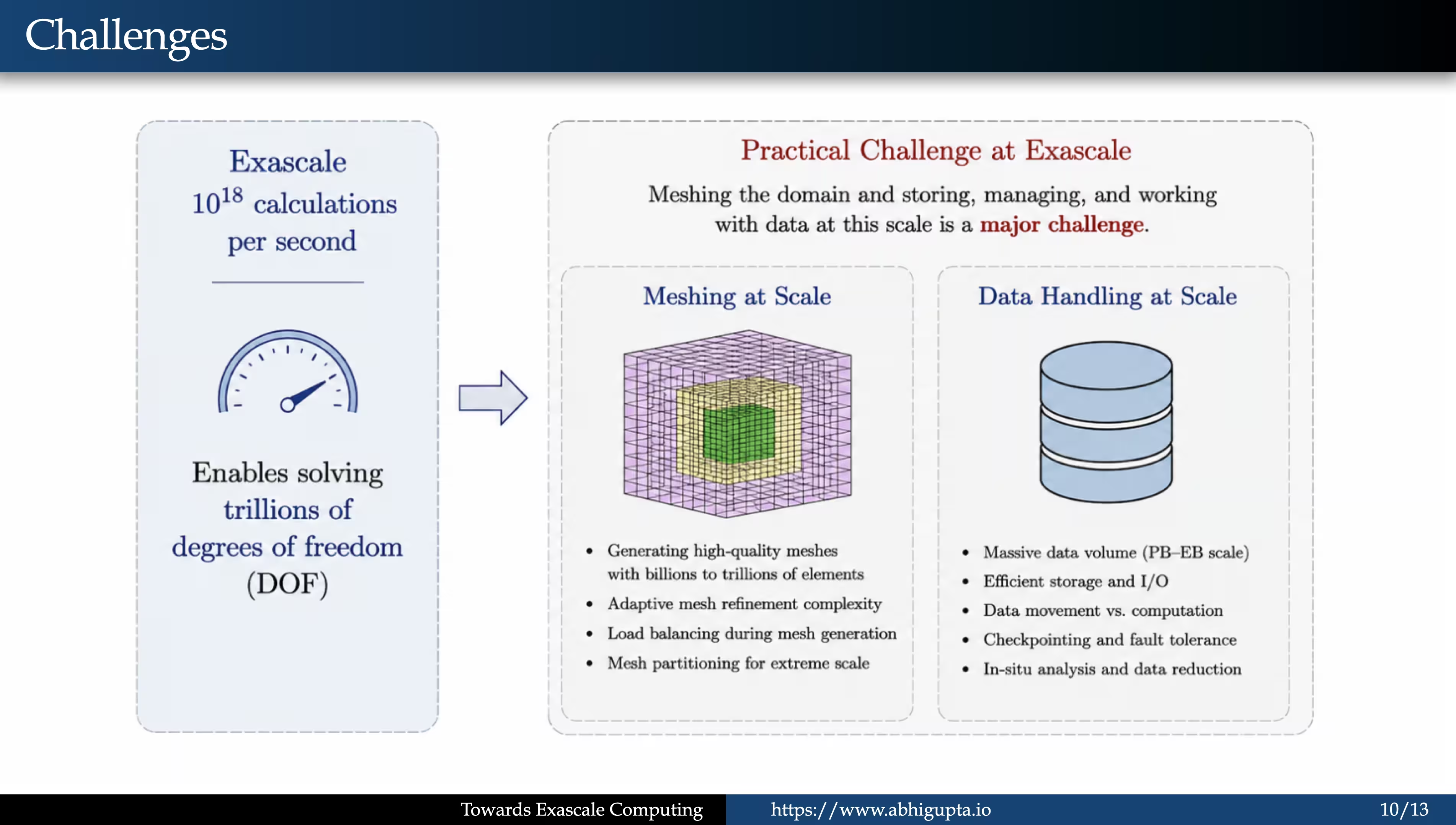Figure 8: Challenges in large-scale computing

Then comes adaptive refinement, load balancing, and mesh partitioning for extreme-scale systems.

The second major challenge is data handling. At exascale, we deal with massive data volumes. We need efficient storage and I/O strategies. If we are designing systems on Google Cloud, AWS, or supercomputers, we must think carefully about how data is written, stored, moved, and reused.

Checkpointing is another critical requirement. We need to save the state of the solution algorithm at different stages so that if something breaks, we can restart the simulation.

At this scale, things are bound to break.

The next hope is to use exascale systems to generate large quantities of data that can train machine learning surrogates. Even though we have large compute resources, we cannot use them indefinitely because they cost millions of dollars to run.

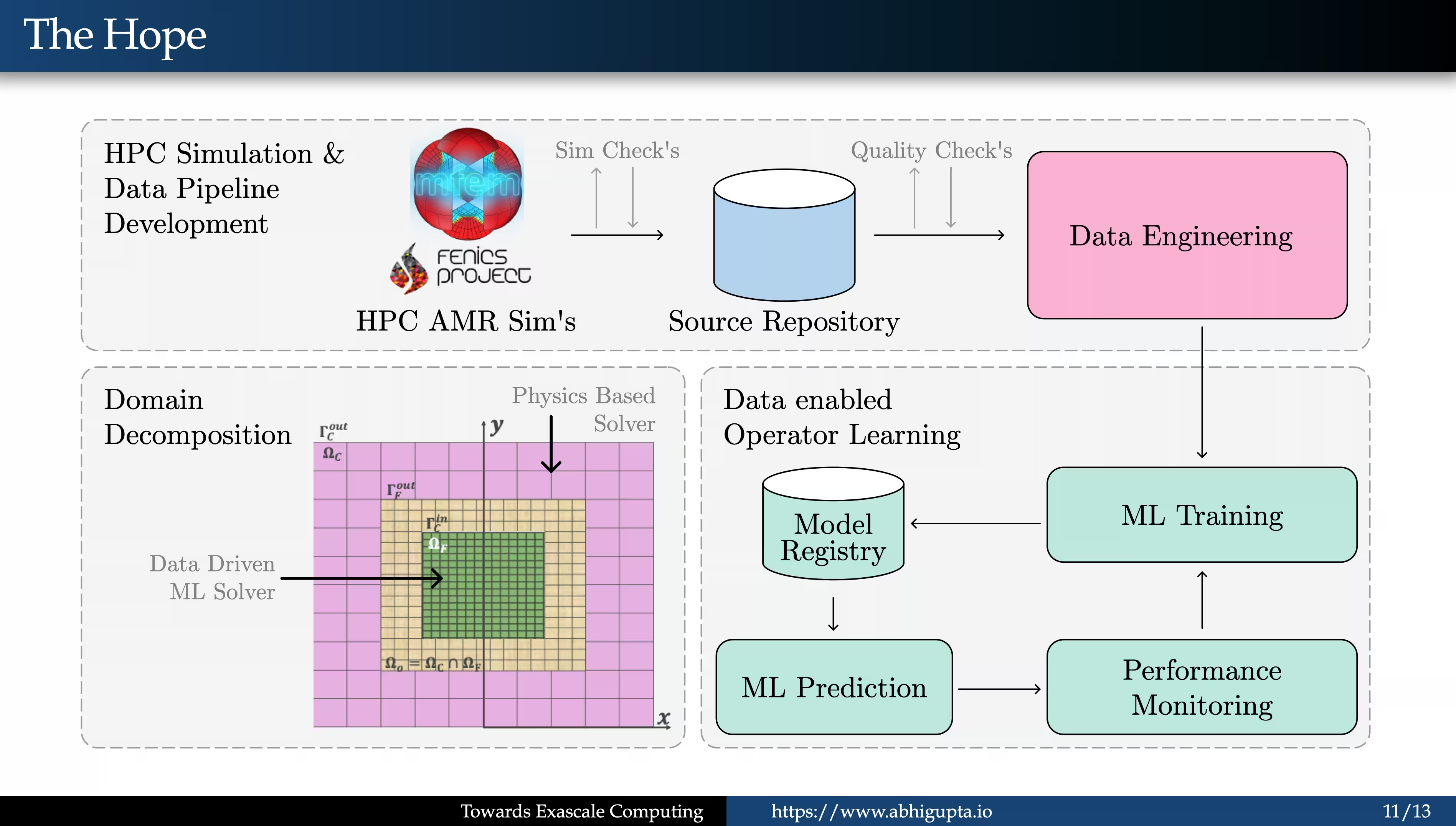Figure 9: The next hope in exascale systems

With scientific machine learning, there is a possibility that we can generate data using exascale systems, train ML surrogates, and reduce inference cost by factors of 10,000 or even 100,000.

If that happens, problems that currently need exascale resources may eventually become solvable on workstations, and perhaps one day even on laptops.

10. Where to Learn

For those interested in learning high-performance computing, parallelization, and framework development, we have packaged these ideas into a short course on FEniCS.

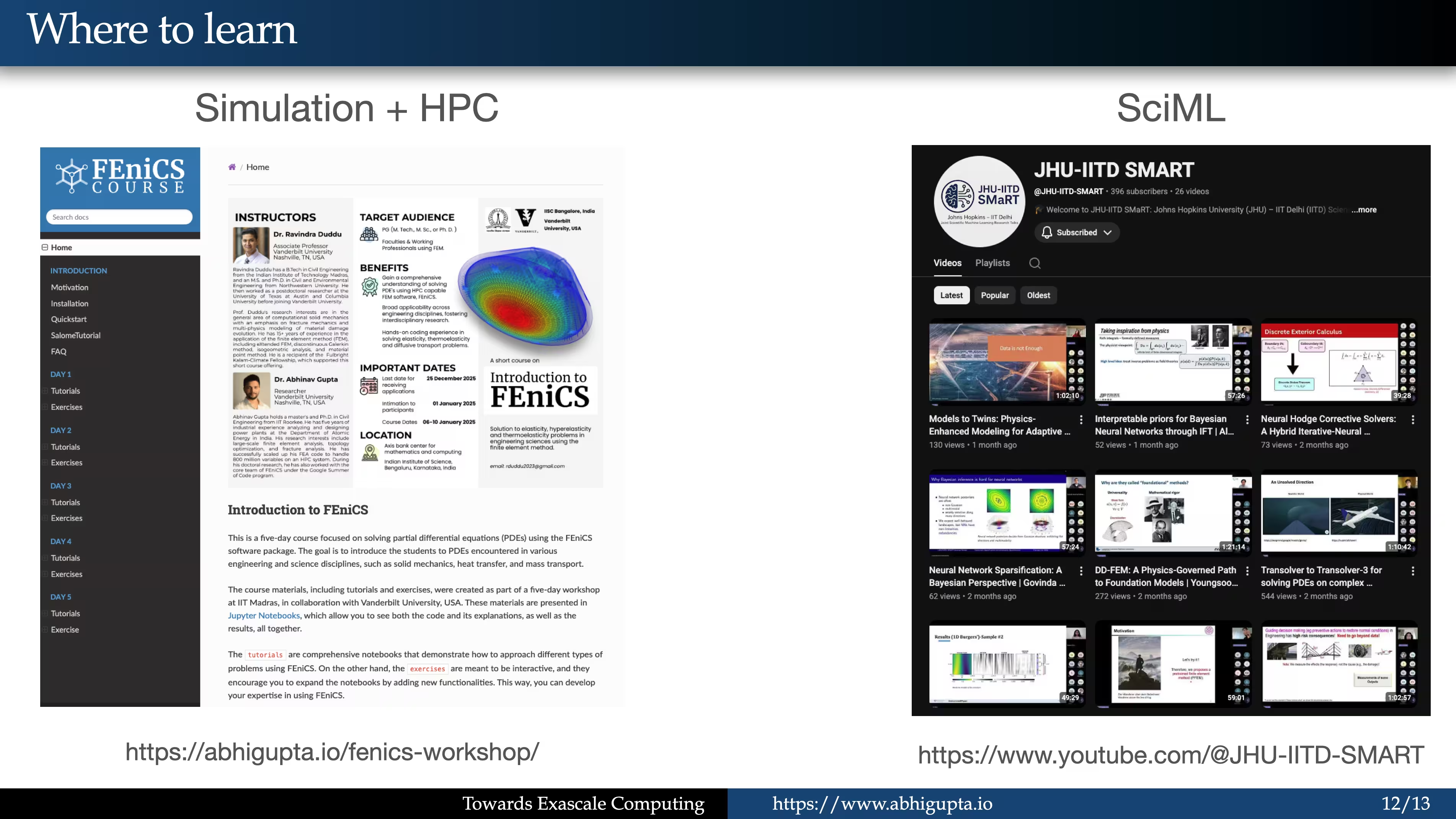Figure 10: Where to get started

If you are interested in developing custom algorithms for simulations, I would recommend looking into:

• FEniCS Project
• MFEM Project

These are excellent places to understand how algorithms are designed for truly industry-grade problems.

If you are interested in scientific machine learning, my collaborators from IIT Delhi and Johns Hopkins University have created a platform where researchers from around the world teach the latest developments in scientific machine learning.

Their YouTube channel is a good place to understand how the field is evolving.

If you have questions, join the Slack community and have conversations with us.

11. Collaboration Oppurtunities

I would like to end by sharing what I believe is the mission of high-performance computing.

The ultimate mission of high-performance computing is to build high-fidelity digital twins of nature, human systems, and engineered infrastructure.

These digital twins can help us achieve predictive understanding, intelligent control, and real-time decision-making.

Imagine having sensors on bridges, buildings, vehicles, or even human bodies before surgery, and then building accurate digital twins that can help us make better decisions in real time.

We are still far away from that reality.

Current simulations still make many approximations. We often assume materials are homogeneous and isotropic. We usually do not work at the level of molecular dynamics. We often simplify complex fluid-structure interactions.

There are still many unsolved challenges.

The work I presented is the result of collaborations with many researchers and institutions. But we need more people to enter this field.

The people who can excel here are those who love computer science, mechanical engineering, and mathematics.

So, if this field resonates with you, come join us. Talk to us. Ask questions. Build algorithms. Explore simulations.

There are many hard problems still waiting to be solved, and the future of scientific computing will be built by those willing to work at the intersection of physics, mathematics, and computation.