viscosity is the important parameter to assess the force fluid is applying of any object. It helps in understanding drag force.

Take three glasses and fill them with water, oil, and honey. Take the eraser from your table, drop it in the above three different glasses one by one, and note the time. What have you observed? The time taken by the eraser to hit the bottom is more for honey when compared with the other two liquids. This is due to the viscosity of the liquid.
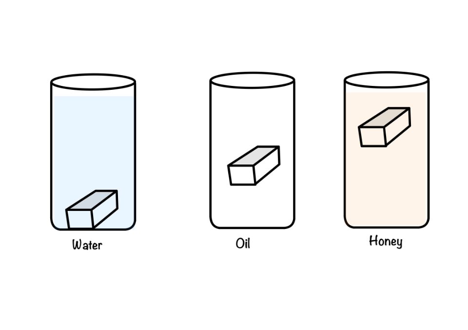
The viscosity resists the relative motion in the liquid. More the viscosity more is the resistance. In this article we will learn about the viscosity of liquid, how to evaluate it, how to calculate the force exerted by the viscosity?
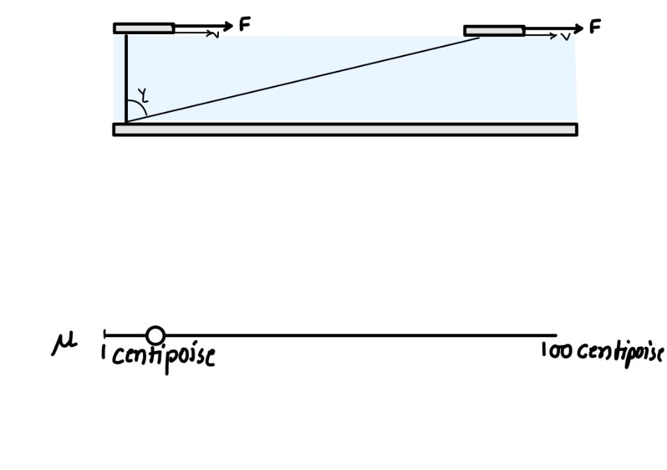
In this interactive widget, you can feel the viscosity by yourself. Let's discuss the setup of the widget. There are two plates. One is a long plate, which is at the bottom. We have placed the movable plate at the top of the water.
When we try to move the upper plate, it will get resistance from the water. More resistance will slow down the movement of the plate. Now slide the button and try the viscosity of your choice you may find more viscosity will increase the timing of the plate. This is how viscosity will control the rate of change of strain.
To calculate the force exerted by the viscosity of the liquid on solid ball lets try to understand this with one simple experiment. Consider two plates and fluid flowing between them. One plate is stationary and another plate which is at the top is moving with the velocity . The velocity profile is linear and hence the velocity at any point can be calculated as:
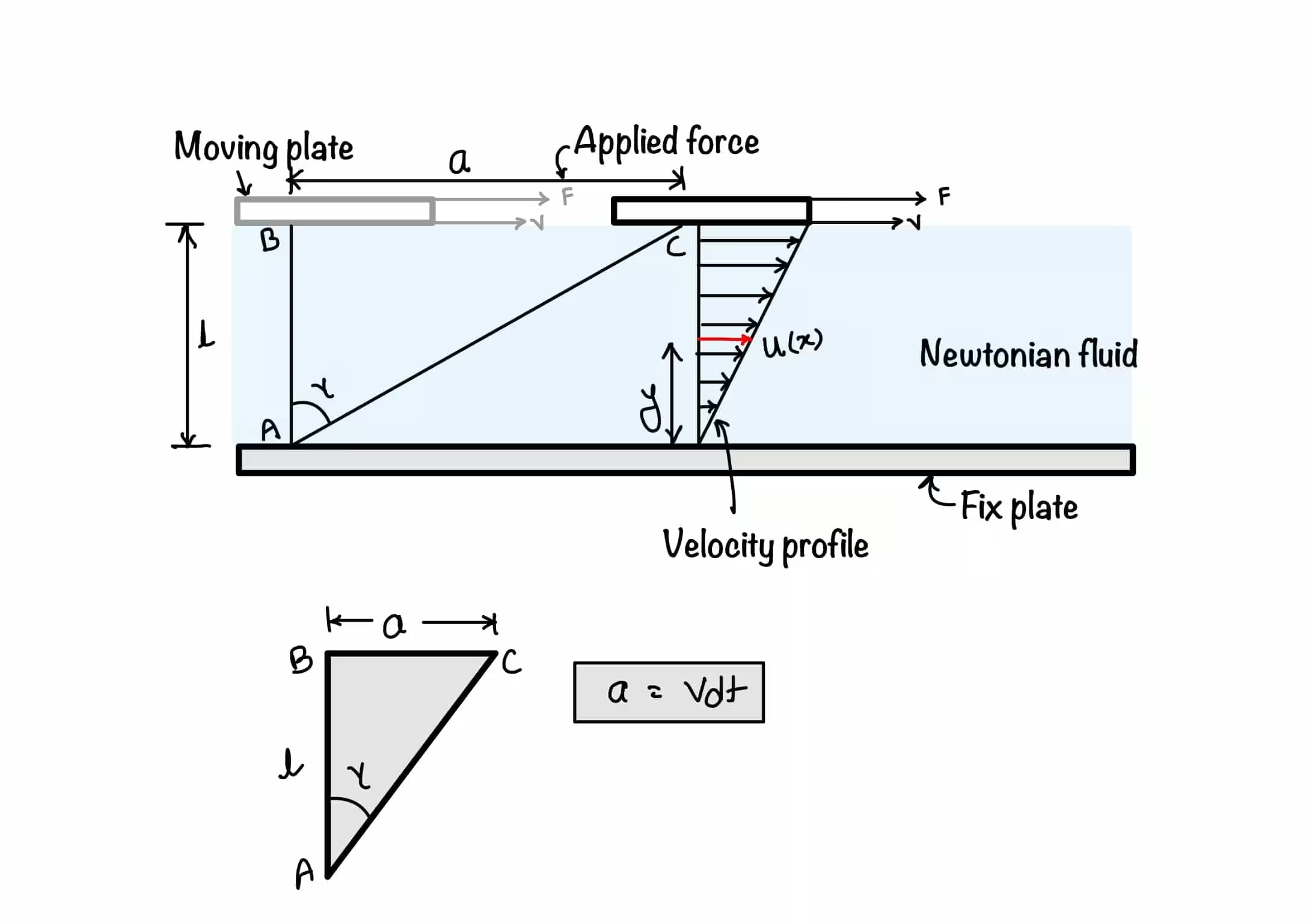
where is the velocity at any point . The force we are applying in the top plate is generating the shear stress . This force is causing the shear deformation in the body. The shear stress is directly proportional to the rate of shear strain.
A similar expression we derive for the solid as well. But the difference between them is liquid has no resistance to shear strain, but shear stress is directly proportional to rate of shear strain, in case of solid the shear stress is directly proportional to shear strain.
In 1687, Sir Isaac Newton proposed the law of viscosity for fluid. It says " the fluid for which velocity gradient is directly proportional to the shear stress are called Newtonian fluids."
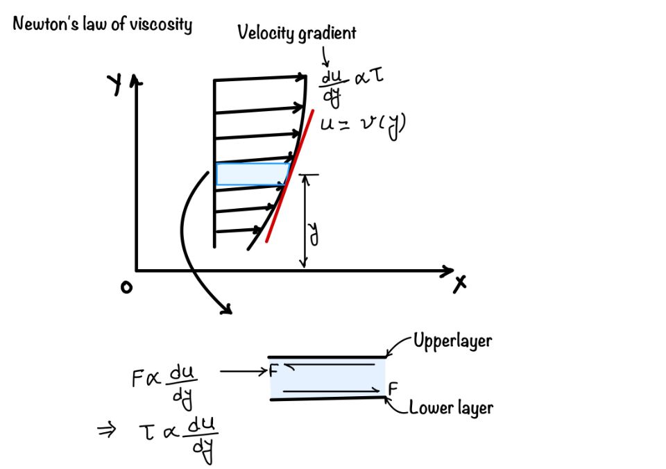
Where is velocity gradient. The rate of change of velocity with respect to distance .
Here, we need some explanation. We have earlier defined the proportionality with rate of deformation and in the Newton's law for viscosity we have written the relation with velocity gradient . How they are related with each other and why we need them?
The viscosity law defined by Newton used the velocity gradient. It says shear stress in the fluid is directly proportional to the velocity gradient of the liquid. This is valid for the simple one-dimensional laminar flow. As you can see from the section above where we have derived the relation between the rate of change of deformation with the velocity gradient of the liquid. This derivation is valid only for the one-dimensional Newtonian fluid.
Based on the definition of Newton's law of viscosity, we can categorize the fluid into different types. The fluids that follow Newton's law of viscosity we call them the Newtonian fluid. The remaining kinds of fluids we call non-Newtonian fluids.
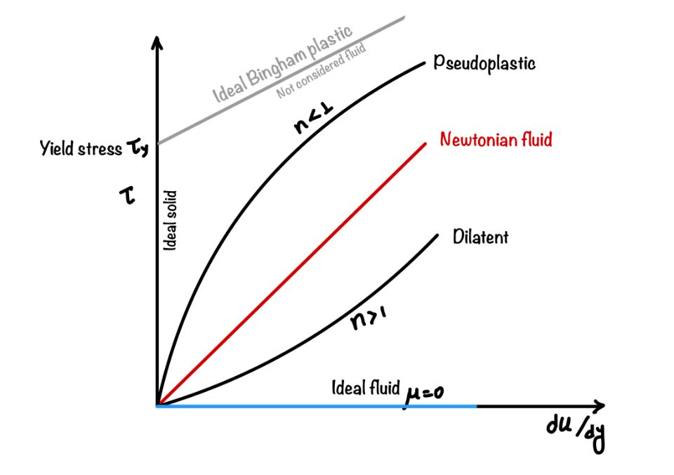
In the graph between the velocity gradient and shear stress we can see the Newtonian and non-Newtonian fluids. We define the ideal fluid here. It has the zero viscosity. Similarly the when shear rate is zero for any force than it is ideal solid.
Let's consider the above experiment again which we have used to explain the viscosity. The shear strain is the angle which is shown in the figure. The force is applied to upper plate which gives the velocity to the plate. If the plate travels the distance at time . The distance between the plate is .
If the angle of deformation is small than
This is how the deformation rate can be related with the velocity gradient.
The fluids which does not follow the Newton's law, we call them as Non-Newtonian fluid. Ostwald-de-waele model gives the power law for Non-Newtonian fluid. Which is as follows:
After some adjustment we can write it as:
Where is the flow behavior index and is the flow consistency index. This is the power law. Many fluids follow this law. For , we call the fluid pseudoplastic fluid. For the fluids that follow the power law for, we call it dilatant fluid.
As the cause of viscosity is the bond between the particles in the fluid and for the gases it is due to collision of particle. When we increase the temperature for the liquid the viscosity reduces as the bond between atoms become weak.
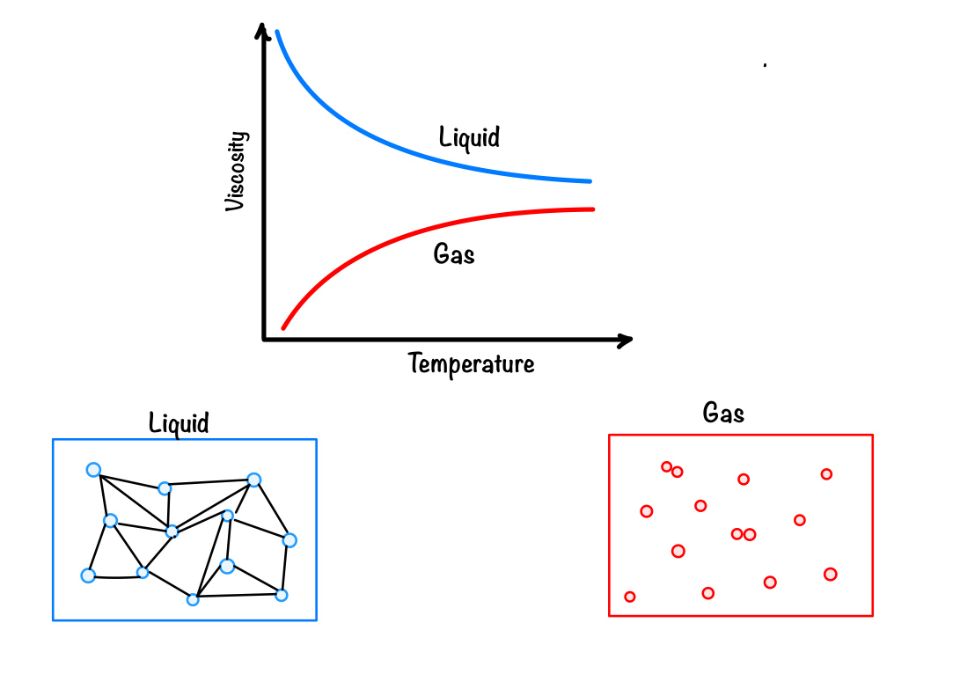
In the case of the gas, the collision increases with an increase in temperature. Hence this increase in temperature increases the viscosity of the gas. You can refer the graph to see the variation of viscosity with temperature.
We define a fluid as an ideal fluid whose viscosity is zero. But generally, all the real fluids have viscosity. Then why do we define the term ideal fluid? It is because at high speed of flow away from the surface of the boundary of the solid there is a zone where fluid can show the behaviour which is similar to the ideal fluid.
Apart from this, we categorise the fluid based on the viscosity. This concept is useful for the calculation of drag force into the solid.
This article explains how we can define the viscosity in the fluid, how it is related to the shear stress and strain of the solid. Apart from this, there are many essential learnings which we can conclude here.
In this blog, you have learned the following points:
Viscosity: According to the simple definition we can define the it as the ratio of shear stress in the fluid to the velocity gradient of the fluid.
Apparent viscosity: In non-Newtonian fluid, we can observe that the viscosity is not only the property of fluid rather it is the property of fluid flow. Hence, we call it apparent viscosity.
Your trusted source for breaking down core engineering concepts using first-principles thinking.