Heat Conduction Equation | Definition & Derivation
The heat conduction equation is a partial differential equation defining the temperature distribution over time and space within a body.
The heat conduction equation generally comes into the picture whenever analysis of a system is subjected to heat conduction. For example, heat conduction through a large plane wall (perpendicular to the surface), the metal plate at the bottom of the iron press (perpendicular to the iron plate), and a cylindrical nuclear fuel palette (radial direction) or an electrical resistance wire (radial direction).
In this post, you will see the heat conduction equation and how it is derived using the simple energy conservation law.
Heat Conduction equation
In physics, the heat conduction equation is a partial differential equation that defines the temperature distribution (temperature field) over time and space within a body subjected to heat conduction.
The generalized form :
∂x2∂2T+∂y2∂2T+∂z2∂2T+kg˙=α1.∂t∂T
or
∇2T+kg˙=α1∂t∂T
here, T is the temperature [K] g is the heat generation per unit volume [Wm-3] k is the thermal conductivity of the material [Wm-1K-1] α is the thermal diffusivity [m2s-1] t is the time [s]
The heat conduction, also known as the Fourier-Biot equation, governs the variation of temperature with space and time under an unsteady state within a homogeneous and isotropic material.
In practical engineering applications, you have to solve heat transfer problems involving complex and irregular geometries subjected to different boundary conditions. For those cases, the applicability of the heat conduction equation becomes crucial. These cases are generally advanced that you can not simply use Fourier's law to find the heat transfer. Therefore for these practical cases, you have to rely on the heat conduction equation in cartesian, cylindrical, or spherical coordinates to get the temperature distribution and heat transfer rate.
Derivation of Heat Conduction equation
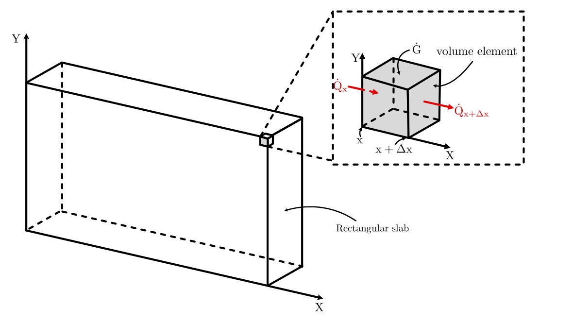
Consider a small cuboidal element of thickness Δx and cross-sectional area A in a large rectangular slab, as shown in the figure below.
Three-dimensional heat conduction across a small volume element.
The slab is homogeneous, having density ρ, the specific heat C, and thermal conductivity k. Based on the law of conservation of energy, the energy balance equation on a small interval of time Δt becomes
Heat conduction rate at x− Heat conduction rate at x+Δx+ Heat generation rate inside the element = Rate of change of the energy content of the element
or
Qx˙−Q˙x+Δx+G˙element=ΔtΔE
Here, Qx is the rate of heat influx, Qx+Δx is the rate of heat efflux, Gelement is the rate of total thermal energy generation within the element, and ΔE is the change in the thermal energy of the element.
Qx˙−Q˙x+Δx+g˙AΔx=ρAΔxCΔtΔT
The term Q x can be expressed with the help of Fourier's law of conduction, and the Qx+Δx term can be defined with Taylor's series expansion. This reduces the above equation to
∂x∂(−kA∂x∂T)∂x+g˙A∂x=ρA∂x.C.∂t∂T
The above equation in three dimension heat conduction becomes
∂x2∂2T+∂y2∂2T+∂z2∂2T+kg˙=α1.∂t∂T
or
∇2T+kg˙=α1∂t∂T
Forms of Heat Conduction equation
The generalized equation as defined above can be simplified into different forms:
Fourier's equation
There is no internal heat generation within the material
∂x2∂2T+∂y2∂2T+∂z2∂2T=α1.∂t∂T
or
∇2T=α1∂t∂T (Fourier’s equation)
Poisson's equation
The heat flows in a steady state
∂x2∂2T+∂y2∂2T+∂z2∂2T+kq˙=0
or
∇2T+kq˙=0(Poisson’s equation)
Laplace equation
The heat flows in a steady state, and there is no internal heat generation within the material
∂x2∂2T+∂y2∂2T+∂z2∂2T=0
or
∇2T=0 (Laplace equation)
Heat Conduction equation in Cylindrical and Spherical coordinate systems
In many engineering cases, there can be the possibility that a particular problem can not be solved using the cartesian coordinate system. The heat conduction equation in cylindrical and spherical coordinates applies in those cases. The generalized heat conduction equations in a cylindrical and spherical coordinate system can be obtained similarly to the cartesian coordinate system, as discussed above. All you need to do in these cases is take volume elements in cylindrical and spherical coordinate systems.
Cylindrical-coordinate
The equation in a cylindrical coordinate system is
The heat conduction equation provides an analytical way to analyze the temperature field within a body. Since it is based on the law of energy conservation, it ensures that it is valid in practical engineering applications.
The key learnings from this post:
Heat conduction equation: The heat conduction equation is a partial differential equation that defines the temperature distribution (temperature field) over time and space within a body subjected to heat conduction. And it is based on energy conservation.
Coordinate systems: It can be defined as cartesian, cylindrical, or spherical coordinate systems.
Forms of conduction equation: There are different forms of it - Fourier's equation, Laplace equation, and Poisson's equation.
Decode scientific breakthroughs using first principles.
Your trusted source for breaking down core engineering concepts using first-principles thinking.