Stability analysis of finite and infinite slope

Slope as show in the Fig 1 may be artificial or natural. Some examples of slopes are cutting, embankment of highways, hillside, valley etc. In all the cases soil want to move from higher point to lower point. This tendency is there because of potential energy. Every structure wants to settle in stable configuration. This tendency of soil movement is called instability. If actual movement of soil occurs then it is called slope failure.

Forces causing the movement of soil may be categorized as follows:

• Gravity force: Due to the weight of the soil. (see the direction of w in fig 1)

• Seepage force: Due to the flow of water through the soil. (refer to seepage flow)

• Earthquake force: In the zone of earthquake-sensitive matter.

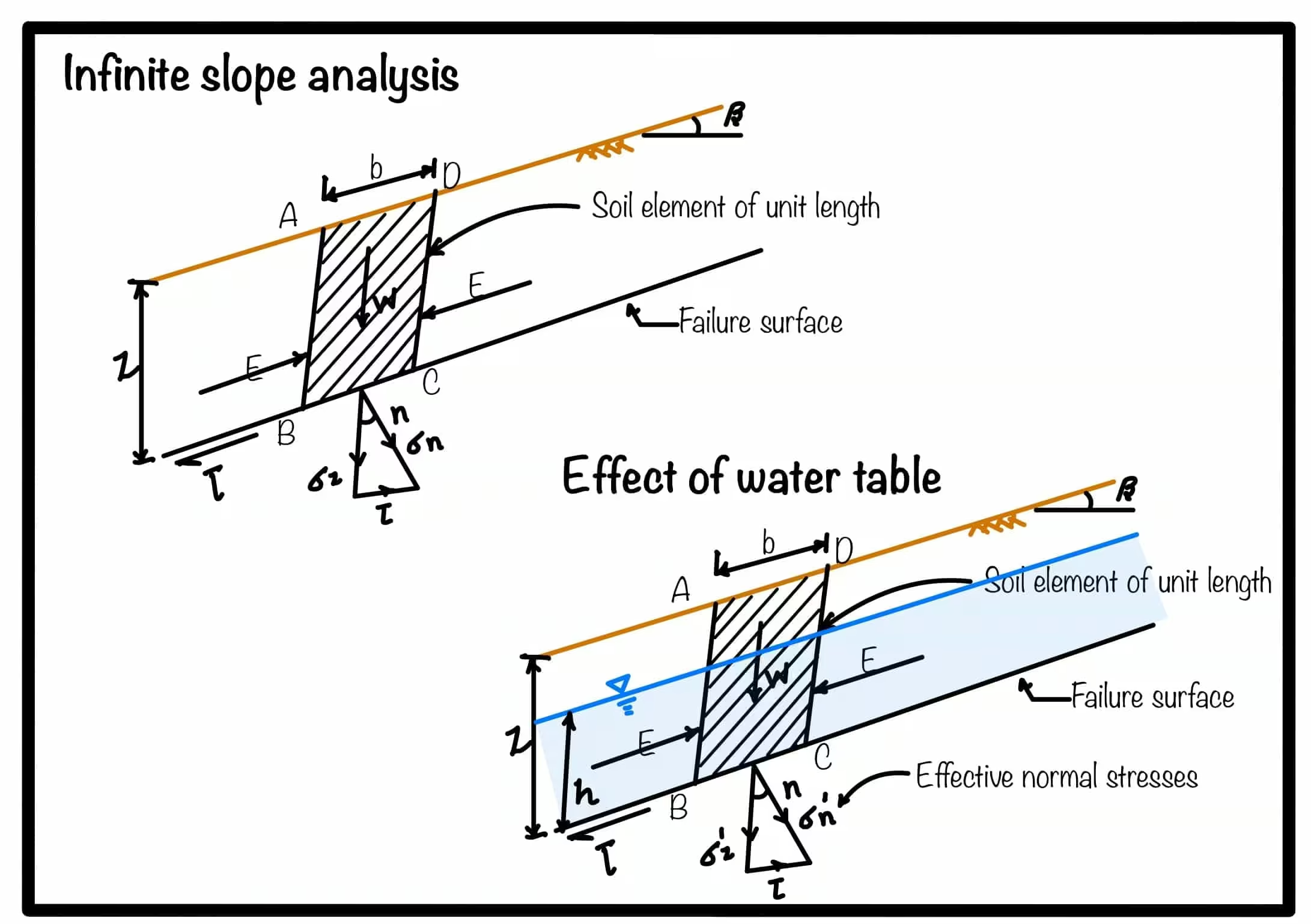
Fig: 1 Stability analysis of infinite slope (a) without water table (b) with water table

Mainly first two forces only causes failure of slope. Earthquake force acts on the seismic zone only. As we have discussed that other soil failure needs analysis of surface. To perform the stability analysis limit equilibrium approach (failure is on the verge of failure) is used along the assumed or known failure surface. This analysis assumes a plane strain condition.

Infinite slopes and stability

What is infinite meaning?

Infinite slope means stresses and soil properties are the same in every vertical plane. And contrary to this there is a term finite slope. Most of the man-made structures like embankment etc. are finite in nature. The failure surface in such a case is a curved surface.

Failure analysis of slope in cohesion-less soil

To analyse the failure in the infinite slope lets discuss the Fig 2 and understand the stress acting and failure surface:

with reference to Fig 2, we can see that the weight of soil block considered is

$W=\gamma z b \cos(\beta)$

Hence the vertical stress (\sigma_{z}) is equal to weight of the soil block. On factorizing the vertical stress (\sigma_z) we can obtain (\sigma_n) and (\tau) as shown in Fig. 2.

Fig:2 Failure analysis of infinite slope with cohesion less soil

Also read: Seepage in soil, permeability of soil

Failure of the wedge as shown in fig 2 will take place when shear stress becomes less than the criteria mentioned in the equation below:

$\tau_f = \sigma_n tan(\phi')$

where, (\tau_f) is the shear stress causing failure, in this case this is the component of stress acting in the (z) direction. (\sigma_n) is the normal component which provides stability to the soil mass and (\phi') is the angle of internal friction which is soil property.

Now, substituting the value of (\tau_f) and (\sigma_n) with component of (\sigma_z):

$\tau_f = \sigma_z \sin(\beta)$

$\sigma_n = \sigma_z \cos(\beta)$

$F=\frac{\tan\phi'}{\tan \beta}$

Note: from this we can conclude that factor of safety of infinite slope in a cohesionless soil is independent of the depth of failure plane. (\phi') is ultimate angle of shearing resistance. If (\beta) is more than the (\phi') slope will become unstable (see the fig 2).

Failure analysis of slope in cohesive soil

When we talk about the cohesive soil, the failure criteria will change. In this case we have cohesion also hence the (c) value will not be zero. Hence in this case failure criteria will be :

$\tau_f = c' + \sigma_n \tan (\phi')$

hence the factor of safety against failure will be :

$F = \frac{\tau_f}{\tau} = \frac{c'+\gamma z \cos^2 (\beta)\tan (\phi')}{\gamma z \cos (\beta) \sin (\beta)}$

In this case both, friction angle (\phi') and (c') governs the failure. Hence if (\beta) is less then (\phi') the also upto certain height slope could be stable. This height is called critical height.

Determination of critical height

For determination of critical height we are going to put F=1 in the above equation and the value of (z) give the critical height:

$1 = \frac{\tau_f}{\tau} = \frac{c'+\gamma z \cos^2 (\beta)\tan (\phi')}{\gamma z \cos (\beta) \sin (\beta)}$

$H_c = \frac{c'}{\gamma (\tan \beta - \tan \phi')cos^2 \beta}$

and if there is the seepage parellel to slope the above equation can modified in the form of :

$H_c = \frac{c'}{\gamma_t (\tan \beta -\frac{\gamma'}{\gamma_t} \tan \phi')cos^2 \beta}$

Finite slope