In this article, we will explore a method for developing a random 3D velocity model using the bottom up approach in Python.

When solving scientific problems, it is important to approach the problem in a systematic and structured manner. One such approach is the bottom up approach, which involves starting from the smallest, most basic components of a problem and gradually building up to a complete solution.
In geophysics, the most common subsurface model is a seismic velocity profile. It is used to understand the subsurface structure of the earth. It helps in the interpretation of seismic data, which is an important tool for exploring and extracting oil, gas, and other subsurface resources. In this article, we will explore a method for developing a random 3D velocity model using the bottom up approach in Python.
The bottom up approach is a step by step approach that starts with a simple model and gradually adds complexity to it. This approach is useful when developing models with a large number of variables, as it allows us to better understand and control the model's behavior.
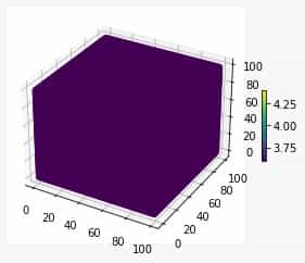
The velocity model we will be developing in this article consists of 100 x 100 x 100 grid points. The basic model has a uniform velocity of 4.0 km/s. It has four stages.
In each of the following four stages, we will add different complexities to the model. So let's understand each stage one by one.
We start with a simple 3D velocity model that represents the average velocity of the subsurface. Use a NumPy array to store the velocities, use matplotlib to manipulate and visualize them. We will use the same plotting code for further steps as well.
import numpy as np
import matplotlib.pyplot as plt
from mpl_toolkits.mplot3d import Axes3D

# Stage 1: Define the basic model
nx, ny, nz = 100, 100, 100
velocity_model = np.ones((nx, ny, nz)) * 4.0

# Plot the velocity model using Matplotlib
fig = plt.figure()
ax = fig.add_subplot(111, projection='3d')
x, y, z = np.meshgrid(np.arange(nx), np.arange(ny), np.arange(nz), indexing='ij')
c=ax.scatter(x.ravel(), y.ravel(), z.ravel(), c=velocity_model.ravel(), cmap='viridis')

ax.set_xlabel('X')
ax.set_ylabel('Y')
ax.set_zlabel('Z')
plt.colorbar(c)
plt.show()
The output of this will be-
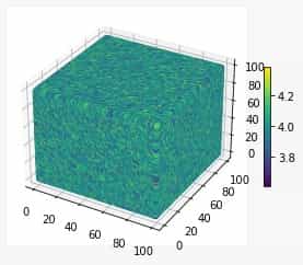
We add heterogeneity to the velocity model by generating random variations in the velocity values. We use NumPy's random module to generate random numbers, which we then use to modify the velocities in the 3D array.
# Stage 2: Add random variations to the model
noise = np.random.uniform(low=-0.1, high=0.1, size=(nx, ny, nz))
velocity_model = velocity_model + noise
Plotting the updated velocity model will give us the following output.
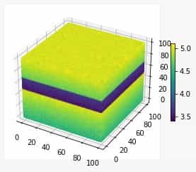
Further, to include more complexity, we add heterogeneity to the model by dividing the single layer into multiple layers with different velocities. The velocity of each layer can be estimated based on well logs or from a combination of geologic and seismic data. This step results in a more realistic velocity model that better reflects the subsurface structures.
# Stage 3: Add horizontal layers to the model
layer_thickness = 20
layer_index = nz // 2
velocity_model[:, :, :layer_index] = velocity_model[:, :, :layer_index] + 0.5
velocity_model[:, :, layer_index:layer_index+layer_thickness] = velocity_model[:, :, layer_index:layer_index+layer_thickness] - 1.0
That will look like-
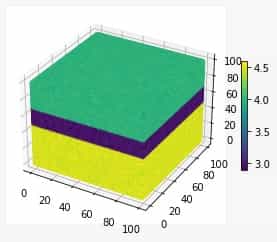
Finally, a vertical gradient is added to the velocity model for providing a more realistic representation of subsurface geology.
# Stage 4: Add vertical variation to the model
vertical_gradient = np.linspace(0, 1, nz)
vertical_gradient = np.tile(vertical_gradient, (nx, ny, 1))
velocity_model = velocity_model + vertical_gradient
This will make our velocity model-
Further complexities can be added for example fault geometries, basin shapes, etc. according to more specific problem.
In this article, we looked at a very simple example of creating a 3D synthetic velocity model using a bottom-up approach. This bottom up approach is a powerful tool that can be applied to many advanced scientific applications. By starting with simple and basic components and gradually adding complexity through multiple stages, this approach allows for a thorough and systematic development of a model.
Key learnings from this post are:
The bottom up approach provides benefits in progress tracking and dealing with complex problems:
By starting with simple and basic components, and gradually adding complexity through multiple stages, it can be useful to visualise the progress at each step.
Bottom up approach is useful to develop a stepwise understanding of a complex problem.
Practical implementation: A 3D subsurface velocity model can be created using the bottom up approach by successively adding features, which simplifies the process and help reach the end goal.
Your trusted source for breaking down core engineering concepts using first-principles thinking.