In this post, you will see how to write Python code for Mohr's circle and the method to find principal stress using that.

Being an engineer, whether civil or mechanical, you will often use Mohr’s circle for finding the stress component at any arbitrary plane. But why not make it fun by writing Python code for Mohr’s circle and principal stress?
In this blog post, you will see Python code for plotting Mohr’s circle and finding the values of principal and maximum shear stresses.
Mohr’s circle represents the transformation laws of the Cauchy stress tensor in graphical form. It helps visualize the normal and shear stress variation with the plane’s orientation.
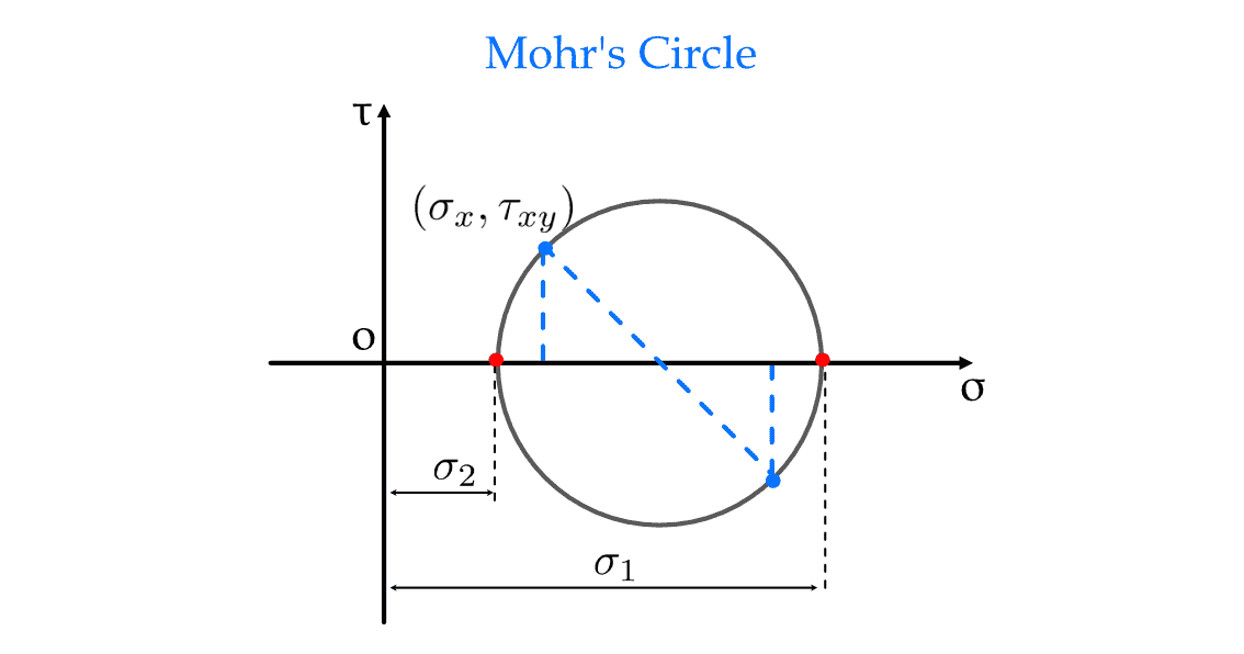
Mohr's circle diagram
Mohr’s circle can also be used to graphically find the location of principal planes and values of principal stresses. Also, you can directly see the value of maximum shear stress, and in-plane maximum shear stresses with Mohr’s circle.
The abscissa and ordinate of each circle point represent the magnitude of normal and shear stress components at a specific orientation. With these values of normal stresses, shear stresses, and principal stress, you can analyze whether any particular structure will fail or not using Theories of Failures.
Principal stress is the normal stress acting on the plane of zero shears, also known as the principal plane. And the principal planes are the planes of zero shear, i.e., there is no shear force acting on these planes.
With these formulas, you can find the value of principal stresses and the location of the principal plane:
There are many approaches for plotting Mohr’s circle using Python programming. The approach used here is first to find the principal stresses and, based on that, calculate the Mohr’s circle’s center and radius.
You can either create a function or define it in terms of a variable. The Python code to calculate the value of principal stresses is:
# Principal and maximum shear stress values
p_stress1 = (sigma_x + sigma_y) / 2 +  (((sigma_x - sigma_y) / 2)**2 + tau_xy **2)**0.5
p_stress2 = (sigma_x + sigma_y) / 2 - (((sigma_x - sigma_y) / 2)**2 + tau_xy **2)**0.5
print("The value of Principal stresses are ",p_stress1 , " and ", p_stress2)
As you already know, the coordinates of Mohr’s circle’s center and radius of Mohr’s circle are:
where σ1 and σ2 are the principal stresses.
radius = (p_stress1 - p_stress2) / 2
center_x = (sigma_x + sigma_y) / 2
center_y = 0

# Store value of circle coordinates in array
X = []
Y = []
X_new = []

for i in np.linspace( 0 , 2 * np.pi , 150 ):
    x = radius * np.cos( i )
    x_new = x + center_x
    y = radius * np.sin( i )

    X.append(x)
    X_new.append(x_new)
    Y.append(y)

# Plot the mohr circle
plt.plot(X_new, Y, color = 'k')
There are two approaches through which you can plot the principal stresses. One approach is based on the actual working practice used for plotting, and the other is a direct approach that marks the points based on the coordinates.
To locate the principal stresses points in Mohr’s circle, you can:
Approach 1: Either take the equation of Mohr’s circle and find its x intersects; the points where it will intersect the X- axis will give the location of maximum and minimum principal stresses.
Approach 2: Or you can mathematically calculate the values of the principal stresses and then locate the corresponding points on the graph. The coordinates of the principal stresses are
The Python code for plotting the principal stresses is:
# Plot principal stress
plt.plot((p_stress1), (0), 'o', color = 'b', label = 'P-stress 1')
plt.plot((p_stress2), (0), 'o', color = 'c', label = 'P-stress 2')
Combining all the above small snippets of code, you get the final code that plots the Mohr’s circle using Python’s Matplotlib library and gives the value of principal stresses.
Key points about the code -
User input: Takes input of the plane stress values from the user.
Principal and maximum shear stress: Calculates the value of the principal stresses and in-plane maximum shear stress. Also principal stresses are highlighted in the plot.
Export plot: Export Mohr’s circle plot into .png and .pdf format.
Labelled plot: The plot is labeled to specify the axes.
Exception handling: Exception handling ensures that the program runs despite the input error.
The complete Python code for finding the values of Principal stresses and plotting Mohr’s circle:
def Mohr_circle():
    try:
        # Take input stress values
        sigma_x = input("Enter the value of axial stress in X direction : ")
        sigma_y = input("Enter the value of axial stress in Y direction : ")
        tau_xy = input("Enter the value of shear stress : ")
        print("\n")

        # Convert str to int
        sigma_x = int(sigma_x)
        sigma_y = int(sigma_y)
        tau_xy = int(tau_xy)

        # Principal and maximum shear stress values
        p_stress1 = (sigma_x + sigma_y) / 2 +  (((sigma_x - sigma_y) / 2)**2 + tau_xy **2)**0.5
        p_stress2 = (sigma_x + sigma_y) / 2 - (((sigma_x - sigma_y) / 2)**2 + tau_xy **2)**0.5
        max_shear = (((sigma_x - sigma_y) / 2)**2 + tau_xy **2)**0.5

        print("\nThe value of Principal stresses are ",p_stress1 , " and ", p_stress2)
        radius = (p_stress1 - p_stress2) / 2
        center_x = (sigma_x + sigma_y) / 2
        center_y = 0

        X = []
        Y = []
        X_new = []

        for i in np.linspace( 0 , 2 * np.pi , 150 ):
            x = radius * np.cos( i )
            x_new = x + center_x
            y = radius * np.sin( i )

            X.append(x)
            X_new.append(x_new)
            Y.append(y)

        # Plot vertical axis
        if radius > 0:
            y_limit = 1.5*radius
        else:
            y_limit = p_stress1*0.5
        a = np.linspace(-y_limit, y_limit,100)
        b = a*0
        plt.plot(b, a, color = 'b', linestyle='dashed')

        # Plot horizontal axis
        if p_stress2 < 0:
            x_limit = p_stress2*1.2

        elif radius == 0 :
            x_limit = -abs(p_stress1)*0.5
        else:
            x_limit = -radius*0.5
        a = np.linspace(x_limit, p_stress1*1.2, 100)
        b = a*0
        plt.plot(a, b, color = 'b', linestyle='dashed')

        # Plot the mohr circle
        plt.plot(X_new, Y, color = 'k')

        # Plot principal stress
        plt.plot((p_stress1), (0), 'o', color = 'b', label = 'P-stress 1')
        plt.plot((p_stress2), (0), 'o', color = 'c', label = 'P-stress 2')

        # Plot the center of Mohr circle
        plt.plot((center_x), (center_y), 'o', color = 'r', label = 'Center')

        plt.xlabel('Sigma X')
        plt.ylabel('Sigma Y')
        plt.title('Mohr Circle')
        plt.legend()

        # Points on circle
        point1 = [sigma_x,tau_xy ]
        point2 = [sigma_y,-tau_xy]

        # Points on the x-axis
        point3 = [sigma_x, 0]
        point4 = [sigma_y, 0]

        # Define point's coordinates for line
        x12_values = [point1[0], point2[0]]
        y12_values = [point1[1], point2[1]]
        x31_values = [point3[0], point1[0]]
        y31_values = [point3[1], point1[1]]
        x42_values = [point4[0], point2[0]]
        y42_values = [point4[1], point2[1]]

        # Plot lines within the circle
        plt.plot(x12_values, y12_values, color = 'g')
        plt.plot(x31_values, y31_values, color = 'g')
        plt.plot(x42_values, y42_values, color = 'g')

        plt.plot()

        # Export plots as png and pdf
        plt.savefig("output/mohr_circle.png")
        plt.savefig("output/mohr_circle.pdf")

    except Exception as e:
        print(e)
        print("Sorry, that's not a valid input !")
The output of this Python code for a particular stress tensor is shown below.
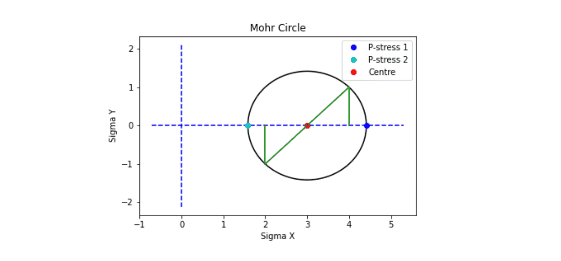
Output of Python code for Mohr's circle
You can try your version of Python code for Mohr’s circle and validate your results through the Mohr’s circle app that is available in the Play store. Mohr’s circle app encompasses all the crucial points related to Mohr’s circle and enables you to evaluate and visualize the value of stresses at any arbitrary plane.
The Python code, as described above, provides the ability to visualize Mohr's circle and find the value of principal and maximum shear stresses.
The key learnings from this post:
Mohr's circle: Mohr’s circle represents the transformation laws of the Cauchy stress tensor in graphical form. It helps visualize the normal and shear stress variation with the plane’s orientation.
Principal stress: Principal stress is the normal stress acting on the plane of zero shears, also known as the principal plane.
Python code for Mohr's circle: Complete code to plot the Mohr's circle that helps in visualizing the variation of stress with plane's orientation.
Your trusted source for breaking down core engineering concepts using first-principles thinking.